December 21, 2018 21 min to read

scRNA-seq下游分析

原理

实验层面

细胞测序需要检测支原体。

简介

相比于bulk RNA-seq，scRNA-seq数据的存在稀疏，高噪声，高维度的特征。

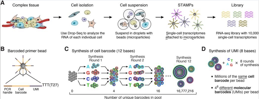
以Nanoliter Droplets方法为例[03]

首先是组织处理得到单细胞，包裹在单个microparticle里面，而microparticle里面又存有包含polyT的beads，于是可以结合mRNA反转成为cDNA，建成pool进行PCR扩增，最后混合所有的STAMPs高通量测序得到数据。

每个micro particle上面的序列由四个部分组成：

一段一样的序列，PCR handle用于后续的PCR扩增
bead特异性的barcode，用来区分单个细胞
UMI，Unique Molecular Identifier，4 - 8bp，用来区分transcripts
30bp的oligo-dT，用来捕捉mRNA完成反转录

问题

扩增偏差，单个细胞初始转录本的捕捉效率和低输入
基因丢失（Gene dropouts），有些基因会在某个细胞里检测到具有中等表达水平却在其它细胞里面没有被发现
tag-based的优势在于它可以结合UMI（前面介绍过）来提高定量的水平，缺点在于未捕捉完全的转录本序列，在比对的时候无法区分iosform (Archer et al. 2016)

实战

简介

S4对象中有一系列的slot变量，其类型就是我们设置的类型，可以为S4对象定义方法。

SingleCellExperiment类是用于单细胞基因组数据的轻量级容器。行代表特征，列代表细胞。SingleCellExperiment类包含：int_elementMetadata，用于保存内部元数据的每行；int_colData，用于保存内部元数据的每列；int_metadata，用于保存内部元数据的全部对象；reducedDims，用于保存降维结果；int_前缀不适合用户直接操作的内部slots。

常用的R包

scater

实操

library(DropletUtils)
library(biomaRt)
library(dplyr)
library(scater)

path="C:\\Users\\Administrator\\Desktop\\hg19"
sce   = read10xCounts(path, col.names=TRUE)
###获取基因注释信息
ensembl = useMart("ensembl",dataset="hsapiens_gene_ensembl")
attr.string = c('ensembl_gene_id', 'hgnc_symbol', 'chromosome_name')
attr.string = c(attr.string, 'start_position', 'end_position', 'strand')
attr.string = c(attr.string, 'description', 'percentage_gene_gc_content')
attr.string = c(attr.string, 'gene_biotype')
rowData(sce)[1:2,]
gene.annotation = getBM(attributes=attr.string, 
                        filters =  'ensembl_gene_id', 
                        values = rowData(sce)$ID, 
                        mart = ensembl)
t1 = table(gene.annotation$ensembl_gene_id)
t2 = t1[t1 > 1]
gene.annotation[which(gene.annotation$ensembl_gene_id %in% names(t2)),]
gene.annotation = distinct(gene.annotation, ensembl_gene_id, 
                           .keep_all = TRUE)
gene.missing = setdiff(rowData(sce)$ID, gene.annotation$ensembl_gene_id)
w2kp = match(gene.annotation$ensembl_gene_id, rowData(sce)$ID)
sce  = sce[w2kp,]
dim(sce)
table(gene.annotation$ensembl_gene_id == rowData(sce)$ID)
rowData(sce)  = gene.annotation
rownames(sce) = uniquifyFeatureNames(rowData(sce)$ensembl_gene_id, 
                                     rowData(sce)$hgnc_symbol)
###Identify low quallity cells
bcrank = barcodeRanks(counts(sce))
# Only showing unique points for plotting speed.
uniq = !duplicated(bcrank$rank)

par(mar=c(5,4,2,1), bty="n")
plot(bcrank$rank[uniq], bcrank$total[uniq], log="xy", 
     xlab="Rank", ylab="Total UMI count", cex=0.5, cex.lab=1.2)

abline(h=bcrank$inflection, col="darkgreen", lty=2)
abline(h=bcrank$knee, col="dodgerblue", lty=2)

legend("left", legend=c("Inflection", "Knee"), bty="n", 
       col=c("darkgreen", "dodgerblue"), lty=2, cex=1.2)
bcrank$inflection
bcrank$knee
summary(bcrank$total)
table(bcrank$total >= bcrank$knee)
table(bcrank$total >= bcrank$inflection)
set.seed(100)
e.out = emptyDrops(counts(sce))
e.out
is.cell = (e.out$FDR <= 0.01)
par(mar=c(5,4,1,1), mfrow=c(1,2), bty="n")
plot(e.out$Total, -e.out$LogProb, col=ifelse(is.cell, "red", "black"),
     xlab="Total UMI count", ylab="-Log Probability", cex=0.2)
abline(v = bcrank$inflection, col="darkgreen")
abline(v = bcrank$knee, col="dodgerblue")
legend("bottomright", legend=c("Inflection", "Knee"), bty="n", 
       col=c("darkgreen", "dodgerblue"), lty=1, cex=1.2)

plot(e.out$Total, -e.out$LogProb, col=ifelse(is.cell, "red", "black"),
     xlab="Total UMI count", ylab="-Log Probability", cex=0.2, xlim=c(0,2000), ylim=c(0,2000))
abline(v = bcrank$inflection, col="darkgreen")
abline(v = bcrank$knee, col="dodgerblue")

table(colnames(sce) == rownames(e.out))
table(e.out$FDR <= 0.01, useNA="ifany")
table(is.cell, e.out$Total >= bcrank$inflection)
w2kp = which(is.cell & e.out$Total >= bcrank$inflection)
sce = sce[,w2kp]
dim(sce)
library(data.table)
ribo.file = "C:\\Users\\Administrator\\Desktop\\ribosome_genes.txt"
ribo = fread(ribo.file)
dim(ribo)


is.mito = which(rowData(sce)$chromosome_name == "MT")
is.ribo = which(rowData(sce)$hgnc_symbol %in% ribo$`Approved symbol`)
length(is.ribo)
sce = calculateQCMetrics(sce, feature_controls=list(Mt=is.mito, Ri=is.ribo))
colnames(colData(sce))
par(mfrow=c(2,2), mar=c(5, 4, 1, 1), bty="n")
hist(log10(sce$total_counts), xlab="log10(Library sizes)", main="", 
     breaks=20, col="grey80", ylab="Number of cells")

hist(log10(sce$total_features), xlab="log10(# of expressed genes)", 
     main="", breaks=20, col="grey80", ylab="Number of cells")

hist(sce$pct_counts_Ri, xlab="Ribosome prop. (%)",
     ylab="Number of cells", breaks=40, main="", col="grey80")

hist(sce$pct_counts_Mt, xlab="Mitochondrial prop. (%)", 
     ylab="Number of cells", breaks=80, main="", col="grey80")


par(mfrow=c(2,2), mar=c(5, 4, 1, 1), bty="n")
smoothScatter(log10(sce$total_counts), log10(sce$total_features), 
              xlab="log10(Library sizes)", ylab="log10(# of expressed genes)", 
              nrpoints=500, cex=0.5)
smoothScatter(log10(sce$total_counts), sce$pct_counts_Ri, 
              xlab="log10(Library sizes)", ylab="Ribosome prop. (%)",
              nrpoints=500, cex=0.5)
abline(h=10,  lty=1)
smoothScatter(log10(sce$total_counts), sce$pct_counts_Mt, 
              xlab="log10(Library sizes)", ylab="Mitochondrial prop. (%)",
              nrpoints=500, cex=0.5)
abline(h=5,  lty=1)
smoothScatter(sce$pct_counts_Ri, sce$pct_counts_Mt, 
              xlab="Ribosome prop. (%)", ylab="Mitochondrial prop. (%)",
              nrpoints=500, cex=0.5)
abline(h=5,  lty=1)
abline(v=10, lty=1)

table(sce$pct_counts_Mt > 5, sce$pct_counts_Ri < 10)
sce.lq = sce[,which(sce$pct_counts_Mt > 5 | sce$pct_counts_Ri < 10)]
sce = sce[,which(sce$pct_counts_Mt <= 5 | sce$pct_counts_Ri >= 10)]

par(mfrow=c(1,3), mar=c(5,4,1,1))
hist(log10(rowData(sce)$mean_counts+1e-6), col="grey80",  main="", 
     breaks=40, xlab="log10(ave # of UMI + 1e-6)")
hist(log10(rowData(sce)$n_cells_by_counts+1), col="grey80", main="", 
     breaks=40, xlab="log10(# of expressed cells + 1)")
smoothScatter(log10(rowData(sce)$mean_counts+1e-6), 
              log10(rowData(sce)$n_cells_by_counts + 1), 
              xlab="log10(ave # of UMI + 1e-6)", 
              ylab="log10(# of expressed cells + 1)")

tb1 = table(rowData(sce)$n_cells_by_counts)
names(rowData(sce))[6] = "strand_n"
sce = sce[which(rowData(sce)$n_cells_by_counts > 1),]
dim(sce)
par(mar=c(5,4,1,1))
od1 = order(rowData(sce)$mean_counts, decreasing = TRUE)
barplot(rowData(sce)$mean_counts[od1[20:1]], las=1, 
        names.arg=rowData(sce)$hgnc_symbol[od1[20:1]], 
        horiz=TRUE, cex.names=0.5, cex.axis=0.7, 
        xlab="ave # of UMI")

library(scran)
clusters = quickCluster(sce, min.mean=0.1, method="igraph")
sce = computeSumFactors(sce, cluster=clusters, min.mean=0.1)
par(mfrow=c(1,2), mar=c(5,4,2,1), bty="n")
smoothScatter(sce$total_counts, sizeFactors(sce), log="xy", 
              xlab="total counts", ylab="size factors")
plot(sce$total_counts, sizeFactors(sce), log="xy", 
     xlab="total counts", ylab="size factors", 
     cex=0.3, pch=20, col=rgb(0.1,0.2,0.7,0.3))
sce = normalize(sce)
new.trend = makeTechTrend(x=sce)
fit = trendVar(sce, use.spikes=FALSE, loess.args=list(span=0.05))

par(mfrow=c(1,1), mar=c(5,4,2,1), bty="n")
plot(fit$mean, fit$var, pch=20, col=rgb(0.1,0.2,0.7,0.6), 
     xlab="log(mean)", ylab="var")
curve(fit$trend(x), col="orange", lwd=2, add=TRUE)
curve(new.trend(x), col="red", lwd=2, add=TRUE)
legend("topright", legend=c("Poisson noise", "observed trend"), 
       lty=1, lwd=2, col=c("red", "orange"), bty="n")

fit$trend = new.trend
dec = decomposeVar(fit=fit)
top.dec = dec[order(dec$bio, decreasing=TRUE),]
plotExpression(sce, features=rownames(top.dec)[1:10])

sce = denoisePCA(sce, technical=new.trend, approx=TRUE)
plot(log10(attr(reducedDim(sce), "percentVar")), xlab="PC",
     ylab="log10(Prop of variance explained)", pch=20, cex=0.6, 
     col=rgb(0.8, 0.2, 0.2, 0.5))
abline(v=ncol(reducedDim(sce, "PCA")), lty=2, col="red")

df_pcs = data.frame(reducedDim(sce, "PCA"))
df_pcs$log10_total_features = colData(sce)$log10_total_features

gp1 = ggplot(df_pcs, aes(PC1,PC2,col=log10_total_features)) + 
  geom_point(size=0.2,alpha=0.6) + theme_classic() + 
  scale_colour_gradient(low="lightblue",high="red") +
  guides(color = guide_legend(override.aes = list(size=3)))
gp1

sce = runTSNE(sce, use_dimred="PCA", perplexity=30, rand_seed=100)
df_tsne = data.frame(reducedDim(sce, "TSNE"))
df_tsne$log10_total_features = colData(sce)$log10_total_features

gp1 = ggplot(df_tsne, aes(X1,X2,col=log10_total_features)) + 
  geom_point(size=0.2,alpha=0.6) + theme_classic() + 
  scale_colour_gradient(low="lightblue",high="red") +
  guides(color = guide_legend(override.aes = list(size=3)))
gp1


library(svd)
library(Rtsne)
dec1 = dec
dec1$bio[which(dec$bio < 1e-8)] = 1e-8
dec1$FDR[which(dec$FDR < 1e-100)] = 1e-100

par(mfrow=c(1,2))
hist(log10(dec1$bio), breaks=100, main="")
hist(log10(dec1$FDR), breaks=100, main="")

w2kp = which(dec$FDR < 1e-10 & dec$bio > 0.01)
sce_sub = sce[w2kp,]

edat = t(as.matrix(logcounts(sce_sub)))
edat = scale(edat)
ppk  = propack.svd(edat,neig=50)
pca = t(ppk$d*t(ppk$u))

df_pcs = data.frame(pca)
df_pcs$log10_total_features = colData(sce_sub)$log10_total_features

df_pcs = data.frame(pca)
df_pcs$log10_total_features = colData(sce_sub)$log10_total_features
gp1 = ggplot(df_pcs, aes(X1,X2,col=log10_total_features)) + 
  geom_point(size=0.2,alpha=0.6) + theme_classic() + 
  scale_colour_gradient(low="lightblue",high="red") +
  guides(color = guide_legend(override.aes = list(size=3)))
gp1

colnames(colData(sce_sub))

set.seed(100)
tsne = Rtsne(pca, pca = FALSE)
df_tsne = data.frame(tsne$Y)
df_tsne$log10_total_features_by_counts = colData(sce_sub)$log10_total_features_by_counts
gp1 = ggplot(df_tsne, aes(X1,X2,col=log10_total_features_by_counts)) + 
  geom_point(size=0.2,alpha=0.6) + theme_classic() + 
  scale_colour_gradient(low="lightblue",high="red") +
  guides(color = guide_legend(override.aes = list(size=3)))
gp1

reducedDims(sce_sub) = SimpleList(PCA=pca, TSNE=tsne$Y)

k10_50_pcs = kmeans(reducedDim(sce_sub, "PCA"), centers=10, 
                    iter.max=150, algorithm="MacQueen")
df_tsne$cluster_kmean = as.factor(k10_50_pcs$cluster)
cols = c("#FB9A99","#FF7F00","yellow","orchid","grey",
         "red","dodgerblue2","tan4","green4","#99c9fb")

gp1 = ggplot(df_tsne, aes(X1,X2,col=cluster_kmean)) + 
  geom_point(size=0.2,alpha=0.6) + theme_classic() + 
  scale_color_manual(values=cols) + 
  guides(color = guide_legend(override.aes = list(size=3)))

gp1

snn.gr   = buildSNNGraph(sce_sub, use.dimred="PCA")
clusters = igraph::cluster_walktrap(snn.gr)