6 min to read
逻辑回归原理及其python实现

- content {:toc}
原理
逻辑回归模型:
$h_{\theta}(x)=\frac{1}{1+e^{-{\theta}^{T}x}}$
逻辑回归代价函数:
$J(\theta)=\frac{1}{m}\sum_{i=1}^{m}Cost(h_{\theta}(x^{(i)}),y^{(i)})$
其中:
$$ Cost(h_{\theta}(x),y)= \begin{cases} -log(h_{\theta}(x))& \text{y=1}\ -log(1-h_{\theta}(x))& \text{y=0} \end{cases} $$
该式子合并后:
$Cost(h_{\theta}(x),y)=-ylog(h_{\theta}(x))-(1-y)log(1-h_{\theta}(x))$
即逻辑回归的代价函数:
$J(\theta)=-\frac{1}{m}[\sum_{i=1}^{m}y^{(i)}logh_{\theta}(x^{(i)})+(1-y^{(i)})log(1-h_{\theta}(x^{(i)}))]$
最小化代价函数,使用梯度下降法(gradient descent)。
Want $min_{\theta}J(\theta):$
Repeat {
$\theta_{j}=\theta_{j}-\alpha\frac{\partial}{\partial\theta_{j}}J(\theta)$
} (simultaneously updata all $\theta_{j}$,$\alpha$为学习率)
即:
Repeat {
$\theta_{j}=\theta_{j}-\alpha\sum_{i=1}^{m}(h_{\theta}(x^{(i)})-y^{(i)})x_{j}^{(i)}$
}
正则化(Regularization)
如果我们有非常多的特征,我们通过学习得到的模型可能能够非常好地适应训练集,但是可能不能推广到新的数据集,我们把这种现象成为过拟合。
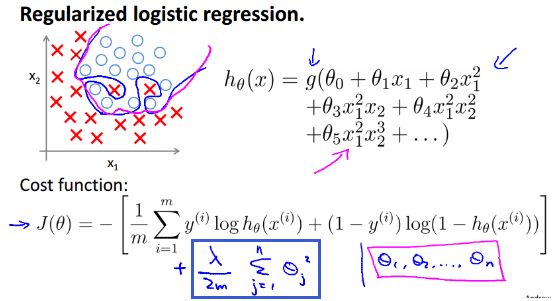
为防止过拟合,提升模型泛化能力,我们需要对所有特征参数(除$\theta_{0}$外)进行惩罚,即保留所有特征,减小参数$\theta$的值,当我们拥有很多不太有用的特征时,正则化会起到很好的作用。
$J(\theta)=-[\frac{1}{m}\sum_{i=1}^{m}(y^{(i)}log(h_{\theta}(x^{(i)}))+(1-y^{(i)})log(1-h_{\theta}(x^{(i)})))]+\frac{\lambda}{2m}\sum_{j=1}^{n}\theta_{j}^{2}$
梯度下降算法:
Repeat until convergence{
$\theta_{0}=\theta_{0}-\alpha\frac{1}{m}\sum_{i=1}^{m}((h_{\theta}(x^{(i)})-y^{(i)})\cdot x_{0}^{(i)})$
$\theta_{j}=\theta_{j}-\alpha\frac{1}{m}\sum_{i=1}^{m}((h_{\theta}(x^{(i)})-y^{(i)})\cdot x_{j}^{(i)}+\frac{\lambda}{m}\theta_{j})$ $for\hspace{1em}j=1,2,...n$
}
python实现
所需数据
代码
# -*- coding:UTF-8 -*-
import matplotlib.pyplot as plt
import numpy as np

"""
函数说明:梯度上升算法测试函数

求函数f(x) = -x^2 + 4x的极大值

Parameters:
	无
Returns:
	无
"""
def Gradient_Ascent_test():
	def f_prime(x_old):									#f(x)的导数
		return -2 * x_old + 4
	x_old = -1											#初始值,给一个小于x_new的值
	x_new = 0											#梯度上升算法初始值,即从(0,0)开始
	alpha = 0.01										#步长,也就是学习速率,控制更新的幅度
	presision = 0.00000001								#精度,也就是更新阈值
	while abs(x_new - x_old) > presision:
		x_old = x_new
		x_new = x_old + alpha * f_prime(x_old)			#上面提到的公式
	print(x_new)										#打印最终求解的极值近似值

"""
函数说明:加载数据

Parameters:
	无
Returns:
	dataMat - 数据列表
	labelMat - 标签列表
"""
def loadDataSet():
	dataMat = []														#创建数据列表
	labelMat = []														#创建标签列表
	fr = open('testSet.txt')											#打开文件
	for line in fr.readlines():											#逐行读取
		lineArr = line.strip().split()									#去回车,放入列表
		dataMat.append([1.0, float(lineArr[0]), float(lineArr[1])])		#添加数据
		labelMat.append(int(lineArr[2]))								#添加标签
	fr.close()															#关闭文件
	return dataMat, labelMat											#返回

"""
函数说明:sigmoid函数

Parameters:
	inX - 数据
Returns:
	sigmoid函数
"""
def sigmoid(inX):
	return 1.0 / (1 + np.exp(-inX))

"""
函数说明:梯度上升算法

Parameters:
	dataMatIn - 数据集
	classLabels - 数据标签
Returns:
	weights.getA() - 求得的权重数组(最优参数)
"""
def gradAscent(dataMatIn, classLabels):
	dataMatrix = np.mat(dataMatIn)										#转换成numpy的mat
	labelMat = np.mat(classLabels).transpose()							#转换成numpy的mat,并进行转置
	m, n = np.shape(dataMatrix)											#返回dataMatrix的大小。m为行数,n为列数。
	alpha = 0.001														#移动步长,也就是学习速率,控制更新的幅度。
	maxCycles = 500														#最大迭代次数
	weights = np.ones((n,1))
	for k in range(maxCycles):
		h = sigmoid(dataMatrix * weights)								#梯度上升矢量化公式
		error = labelMat - h
		weights = weights + alpha * dataMatrix.transpose() * error
	return weights.getA()												#将矩阵转换为数组,返回权重数组

"""
函数说明:绘制数据集

Parameters:
	无
Returns:
	无
"""
def plotDataSet():
	dataMat, labelMat = loadDataSet()									#加载数据集
	dataArr = np.array(dataMat)											#转换成numpy的array数组
	n = np.shape(dataMat)[0]											#数据个数
	xcord1 = []; ycord1 = []											#正样本
	xcord2 = []; ycord2 = []											#负样本
	for i in range(n):													#根据数据集标签进行分类
		if int(labelMat[i]) == 1:
			xcord1.append(dataArr[i,1]); ycord1.append(dataArr[i,2])	#1为正样本
		else:
			xcord2.append(dataArr[i,1]); ycord2.append(dataArr[i,2])	#0为负样本
	fig = plt.figure()
	ax = fig.add_subplot(111)											#添加subplot
	ax.scatter(xcord1, ycord1, s = 20, c = 'red', marker = 's',alpha=.5)#绘制正样本
	ax.scatter(xcord2, ycord2, s = 20, c = 'green',alpha=.5)			#绘制负样本
	plt.title('DataSet')												#绘制title
	plt.xlabel('X1'); plt.ylabel('X2')									#绘制label
	plt.show()															#显示

"""
函数说明:绘制数据集

Parameters:
	weights - 权重参数数组
Returns:
	无
"""
def plotBestFit(weights):
	dataMat, labelMat = loadDataSet()									#加载数据集
	dataArr = np.array(dataMat)											#转换成numpy的array数组
	n = np.shape(dataMat)[0]											#数据个数
	xcord1 = []; ycord1 = []											#正样本
	xcord2 = []; ycord2 = []											#负样本
	for i in range(n):													#根据数据集标签进行分类
		if int(labelMat[i]) == 1:
			xcord1.append(dataArr[i,1]); ycord1.append(dataArr[i,2])	#1为正样本
		else:
			xcord2.append(dataArr[i,1]); ycord2.append(dataArr[i,2])	#0为负样本
	fig = plt.figure()
	ax = fig.add_subplot(111)											#添加subplot
	ax.scatter(xcord1, ycord1, s = 20, c = 'red', marker = 's',alpha=.5)#绘制正样本
	ax.scatter(xcord2, ycord2, s = 20, c = 'green',alpha=.5)			#绘制负样本
	x = np.arange(-3.0, 3.0, 0.1)
	y = (-weights[0] - weights[1] * x) / weights[2]
	ax.plot(x, y)
	plt.title('BestFit')												#绘制title
	plt.xlabel('X1'); plt.ylabel('X2')									#绘制label
	plt.show()

if __name__ == '__main__':
	dataMat, labelMat = loadDataSet()
	weights = gradAscent(dataMat, labelMat)
	plotBestFit(weights)
Comments