7 min to read
几种常见回归及scikit-learn实现

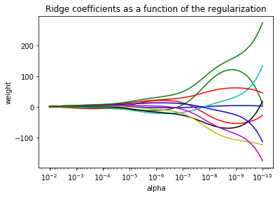
岭回归(Ridge Regression)
原理
岭回归损失函数在线性回归损失函数的基础上增加L2范数惩罚项。
$$ J(\theta)=\frac{1}{2n}\sum_{i=i}^n(y_i-\sum_{j=0}^m\theta_jx_{ij})^2+\lambda\sum_{j=0}^m\theta_j^2 $$
通过确定$\lambda$的值,可以使方差和偏差之间取得平衡。随着$\lambda$的增大,模型方差减小而偏差增大。
特点
可用于解决,样本量小于特征数或者特征之间存在相关的问题。
代码
import numpy as np
import matplotlib.pyplot as plt
from sklearn import linear_model
#构造一个hilbert矩阵10*10
X = 1. / (np.arange(1,11) + np.arange(0,10)[:,np.newaxis])
y = np.ones(10) #10个1

n_alphas = 200
alphas = np.logspace(-10,-2,n_alphas) #等比数列,200个,作为岭回归的系数
clf = linear_model.Ridge(fit_intercept=False)
coefs = []
for a in alphas:
	clf.set_params(alpha=a)
	clf.fit(X,y)
	coefs.append(clf.coef_) #得到200个不同系数所训练出常数参数值

ax = plt.gca()
ax.set_color_cycle(['b', 'r', 'g', 'c', 'k', 'y', 'm'])
ax.plot(alphas,coefs)
ax.set_xscale('log') #转为极坐标系
ax.set_xlim(ax.get_xlim()[::-1]) #反转x轴
plt.xlabel('alpha')
plt.ylabel('weight')
plt.title('Ridge coefficients as a function of the regularization')
plt.axis('tight')
plt.show()
结果展示
Lasso回归
原理
Lasso回归损失函数在线性回归损失函数的基础上增加L1范数惩罚项。
$$ J(\theta)=\frac{1}{2n}\sum_{i=i}^n(y_i-\sum_{j=0}^m\theta_jx_{ij})^2+\lambda\sum_{j=0}^m|\theta_j| $$
特点
Lasso回归能够使得损失函数中的许多θ均变成0,这点要优于岭回归,因为岭回归是要所有的θ均存在的,这样计算量Lasso回归将远远小于岭回归。
代码
import numpy as np
import matplotlib.pyplot as plt
from sklearn.metrics import r2_score
#我们先手动生成一些稀疏数据
print(np.random.seed(42))
n_samples, n_features = 50, 200
X = np.random.randn(n_samples, n_features)
coef = 3 * np.random.randn(n_features) #这个就是实际的参数
inds = np.arange(n_features)
np.random.shuffle(inds) #打乱
coef[inds[10:]] = 0 #生成稀疏数据
y = np.dot(X, coef) #参数与本地点乘
#来点噪音
y += 0.01 * np.random.normal((n_samples,))

X_train, y_train = X[:n_samples//2], y[:n_samples//2]   #除法产生的数据类型是浮点,会报错,将'/'改为'//'
X_test, y_test = X[n_samples//2:], y[n_samples//2:]

from sklearn.linear_model import Lasso
alpha = 0.1
lasso = Lasso(alpha=alpha)

y_pred_lasso = lasso.fit(X_train,y_train).predict(X_test)
r2_score_lasso = r2_score(y_test, y_pred_lasso) #这里是0.38
print(lasso)
print("r2_score's result is %f" % r2_score_lasso)

plt.plot(lasso.coef_, label='Lasso coefficients')
plt.plot(coef, '--', label='original coefficients')
plt.legend(loc="best")
plt.title("Lasso R^2: %f"
          % (r2_score_lasso))
plt.show()
#### 结果展示

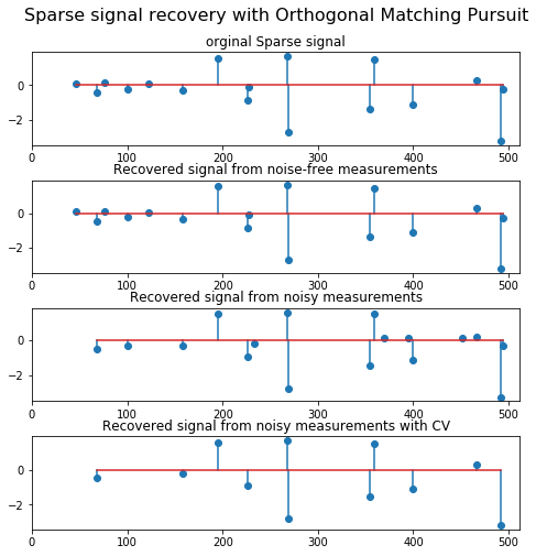
## 正交匹配追踪(Orthogonal Matching Pursuit )
#### 代码
```python
import matplotlib.pyplot as plt
import numpy as np
from sklearn.linear_model import OrthogonalMatchingPursuit
from sklearn.linear_model import OrthogonalMatchingPursuitCV
from sklearn.datasets import make_sparse_coded_signal
n_components, n_features = 512, 100
n_nonzero_coefs = 17
y, X, w = make_sparse_coded_signal(n_samples=1,
n_components=n_components,
n_features=n_features,
n_nonzero_coefs=n_nonzero_coefs,
random_state=0)
idx, = w.nonzero()
y_noise = y + 0.05 * np.random.randn(len(y))
plt.figure(figsize=(7,7))
plt.subplot(4,1,1)
plt.xlim(0,512)
plt.title("orginal Sparse signal")
plt.stem(idx, w[idx])
opm = OrthogonalMatchingPursuit(n_nonzero_coefs=n_nonzero_coefs)
opm.fit(X,y)
coef = opm.coef_
idx_r, = coef.nonzero()
plt.subplot(4, 1, 2)
plt.xlim(0, 512)
plt.title("Recovered signal from noise-free measurements")
plt.stem(idx_r, coef[idx_r])
opm.fit(X, y_noise)
coef = opm.coef_
idx_r, = coef.nonzero()
plt.subplot(4, 1, 3)
plt.xlim(0, 512)
plt.title("Recovered signal from noisy measurements")
plt.stem(idx_r, coef[idx_r])
opm_cv = OrthogonalMatchingPursuitCV()
opm_cv.fit(X,y_noise)
coef = opm_cv.coef_
idx_r, = coef.nonzero()
plt.subplot(4, 1, 4)
plt.xlim(0, 512)
plt.title("Recovered signal from noisy measurements with CV")
plt.stem(idx_r, coef[idx_r])
plt.subplots_adjust(0.06, 0.04, 0.94, 0.90, 0.20, 0.38)
plt.suptitle('Sparse signal recovery with Orthogonal Matching Pursuit',
fontsize=16)
plt.show()
结果展示
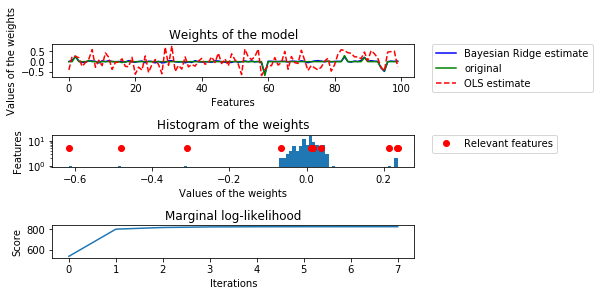
贝叶斯岭回归
代码
import numpy as np
import matplotlib.pyplot as plt
from scipy import stats
from sklearn.linear_model import BayesianRidge, LinearRegression

n_samples, n_features = 100, 100
X = np.random.randn(n_samples, n_features)  # Create Gaussian data
# Create weigts with a precision lambda_ of 4.
lambda_ = 4.
w = np.zeros(n_features)
# Only keep 10 weights of interest
relevant_features = np.random.randint(0, n_features, 10) #找10个随机位置
for i in relevant_features:
    w[i] = stats.norm.rvs(loc=0, scale=1. / np.sqrt(lambda_)) #制造10个非0的特征
# Create noise with a precision alpha of 50.
alpha_ = 50.
noise = stats.norm.rvs(loc=0, scale=1. / np.sqrt(alpha_), size=n_samples)
y = np.dot(X, w) + noise #加噪音

clf = BayesianRidge(compute_score=True)
clf.fit(X,y)

ols = LinearRegression()
ols.fit(X,y)

plt.figure()
plt.subplot(3,1,1)
plt.title("Weights of the model")
plt.plot(clf.coef_, 'b-', label="Bayesian Ridge estimate")
plt.plot(w, 'g-', label="original")
plt.plot(ols.coef_, 'r--', label="OLS estimate")
plt.xlabel("Features")
plt.ylabel("Values of the weights")
plt.legend(bbox_to_anchor=(1.05, 1), loc=2, borderaxespad=0.)

plt.subplot(3,1,2)
plt.title("Histogram of the weights")
plt.hist(clf.coef_, bins=n_features, log=True)
plt.plot(clf.coef_[relevant_features], 5 * np.ones(len(relevant_features)), 'ro', label="Relevant features")
plt.ylabel("Features")
plt.xlabel("Values of the weights")
plt.legend(bbox_to_anchor=(1.05, 1), loc=2, borderaxespad=0.)

plt.subplot(3,1,3)
plt.title("Marginal log-likelihood")
plt.plot(clf.scores_)
plt.ylabel("Score")
plt.xlabel("Iterations")
plt.tight_layout()  #避免图像重叠
plt.show()
结果展示
其他
Elastic Net(弹性网络)是一种使用 L1, L2 范数作为先验正则项训练的线性回归模型。 这种组合允许学习到一个只有少量参数是非零稀疏的模型,就像 Lasso 一样,但是它仍然保持一些像 Ridge 的正则性质。
其他回归包括鲁棒回归、多项式回归、最小角回归。
参考资料
[1]. scikit-learn 学习笔记(一)

Comments