November 6, 2018 10 min to read

使用oligo包处理基因芯片数据

基因芯片数据下载

到GEO官网下载前列腺癌基因芯片数据，包括PCa（GSM1060629、GSM1060630）和PCa bone metastasis（GSM1060627、GSM1060628、GSM1060631、GSM1060632）。下载基因芯片注释文件（GSE43332_family.soft.gz）。

数据预处理

source("https://bioconductor.org/biocLite.R")
biocLite("oligo")
library("oligo")
library("ggplot2")
setwd("F:/ll/GEO/3")
#文件读取
data.dir <- "F:/ll/GEO/3"
##Affymetrix
celfiles <- list.files(data.dir, "\\.gz$")
data.raw <- read.celfiles(filenames = file.path(data.dir, celfiles))
#信息修改
treats <- strsplit("PCa_bone_metastasis PCa_bone_metastasis PCa PCa PCa_bone_metastasis PCa_bone_metastasis", " ")[[1]]
snames <- strsplit("PCa_bone_metastasis1 PCa_bone_metastasis2 PCa1 PCa2 PCa_bone_metastasis3 PCa_bone_metastasis4", " ")[[1]]
#treats <- rep(c("PCa","normal"),c(22,4))
#snames <- c(paste("PCa",1:22,sep = ""),paste("normal",1:4,sep = ""))
sampleNames(data.raw) <- snames
pData(data.raw)$index <- treats
#表达量计算
data.eset <- oligo::rma(data.raw)  #含背景处理、归一化和表达量计算
data.exprs <- exprs(data.eset)  #提取表达量矩阵
#P/A过滤
xpa <- paCalls(data.raw)
AP <- apply(xpa, 1, function(x) any(x < 0.05))  #p值，是指探针表达量与背景相同的概率，越小说明探针与背景的差异越显著，也就是指探针表达的可能性越大。
xids <- as.numeric(names(AP[AP]))
pinfo <- getProbeInfo(data.raw)
#id转换
fids <- pinfo[pinfo$fid %in% xids, 2]  
data.exprs <- data.exprs[rownames(data.exprs) %in% fids, ]
##Affymetrix
##illumina
fileName <- 'GSE38714_non-normalized.txt'
x.lumi <- lumiR.batch(fileName) 
pData(phenoData(x.lumi))
lumi.N.Q <- lumiExpresso(x.lumi)
dataMatrix <- exprs(lumi.N.Q)
##illumina
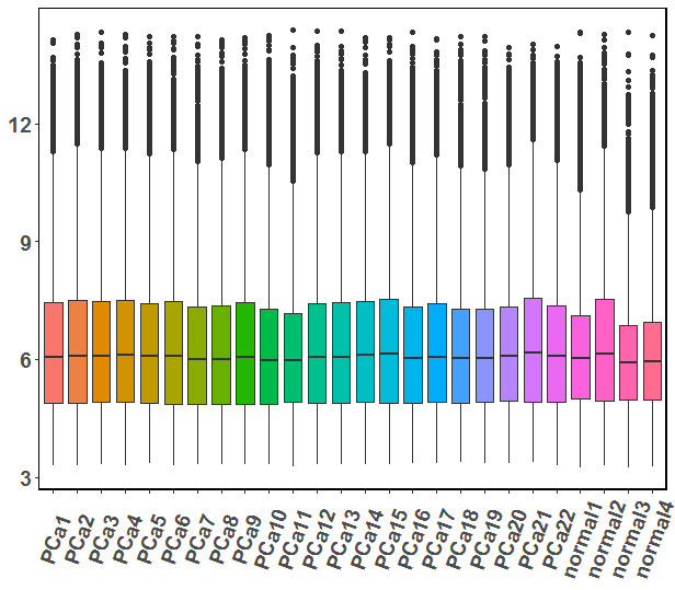
data.exprs.melt <- melt(data.exprs,id.vars = 1)
ggplot(data.exprs.melt, aes(x=Var2, y=value),color=Var2) + 
  geom_boxplot(aes(fill=factor(Var2))) + 
  theme(axis.text.x=element_text(angle=50,hjust=0.5, vjust=0.5,size=14,face="bold"),
        axis.text.y=element_text(size=14,face="bold"),
        panel.background = element_rect(fill = "transparent",colour = NA), 
        panel.grid.minor = element_blank(),
        panel.border=element_rect(colour = "black", fill=NA, size=1) ) +
  labs(y=NULL)+
  theme(legend.position="none") 
id2symbol<-read.csv("id2symbol.csv",header=TRUE,sep=",")
data.exprs2<-cbind(data.exprs,ID=rownames(data.exprs))
data.exprs3<-merge(data.exprs2,id2symbol,by="ID")
write.csv(data.exprs3,"data.exprs3.csv")

探针ID转基因symbol

重复的基因取平均值的最大值的探针

import numpy as np
import pandas as pd
import os

os.getcwd() #获取当前工作目录
os.chdir("F:\\ll\\GEO\\3.1")  #改变当前工作目录
data = pd.read_csv("data.exprs3.csv") #读取数据
data2=data.drop_duplicates('gene_symbol',keep= False )  #保留不重复的数据
index1=list(set(data.index.values).difference(set(data2.index.values)))  #取差集
data3=data.loc[index1]  #保留重复数据
data3['mean']=data3.iloc[:,1:27].mean(1)  #计算平均值
index2=data3.groupby('gene_symbol')['mean'].transform(max)==data3['mean'] #分组求最大值索引
data4=data3[index2]
data5=data4.drop_duplicates('gene_symbol',keep='first')  #进一步去重
data6=data5.iloc[:,0:28]
data7=pd.concat([data2,data6],axis=0)  #合并数据
data7.to_csv('data.exprs3.clear.csv')
"""
index3=list(set(data4.index.values).difference(set(data5.index.values))) 
data8=data.loc[index3]
data9=data8.drop_duplicates('gene_symbol',keep='first')
"""

寻找差异基因

data.exprs3.clear<-read.csv("data.exprs3.clear.csv",header=T,sep=",")
data.exprs3.clear1<-data.exprs3.clear[,2:27]
rownames(data.exprs3.clear1)<-data.exprs3.clear$gene_symbol
library(limma)
#构建试验设计矩阵
design <- model.matrix(~0 + treats)
colnames(design) <- gsub("treats", "", colnames(design))
rownames(design) <- snames
#获取拟合模型
fit1 <- lmFit(data.exprs3.clear1, design)
#组间比较
contrast.matrix <- makeContrasts("PCa-PCa_bone_metastasis", levels = design)
fit2 <- contrasts.fit(fit1, contrast.matrix)
fit2 <- eBayes(fit2)
#获取表达变化倍数和相关统计值
result.all <- topTable(fit2, coef = 1, adjust.method = "fdr", number = 3e+05)
result.diff <- result.all[result.all$adj.P.Val<0.05  & abs(result.all$logFC)>1,]
write.csv(result.all,"result.all.csv")
write.csv(result.diff,"result.diff.csv")

绘图

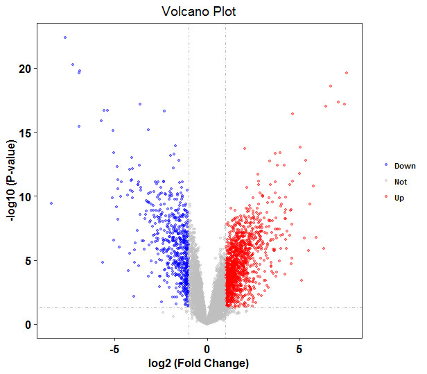
火山图

library(ggplot2)
diff<-read.csv(file="result.all.csv",header=TRUE,sep=",")
diff$threshold = as.factor(ifelse(diff$logFC >=1  & diff$adj.P.Val< 0.05, 'Up', ifelse(diff$adj.P.Val< 0.05 & diff$logFC <= -1, 'Down', 'Not')))
ggplot(data=diff, aes(x=logFC, y=-log10(adj.P.Val), colour=threshold, fill=threshold)) + 
  scale_color_manual(values=c("blue", "grey","red"))+
  geom_point(alpha=0.4, size=1.2) +
  # xlim(c(-4, 4)) +
  # ylim(c(0, 7.5)) +
  theme_bw(base_size = 12, base_family = "Times") +
  geom_vline(xintercept=c(-1,1),lty=4,col="grey",lwd=0.6)+
  geom_hline(yintercept = -log10(0.05),lty=4,col="grey",lwd=0.6)+
  theme(legend.position="right",
        panel.grid=element_blank(),
        legend.title = element_blank(),
        legend.text= element_text(face="bold", color="black",family = "Times", size=8),
        plot.title = element_text(hjust = 0.5),
        axis.text.x = element_text(face="bold", color="black", size=12),
        axis.text.y = element_text(face="bold", color="black", size=12),
        axis.title.x = element_text(face="bold", color="black", size=12),
        axis.title.y = element_text(face="bold",color="black", size=12))+
  labs(x="log2 (Fold Change)",y="-log10 (P-value)",title="Volcano Plot")

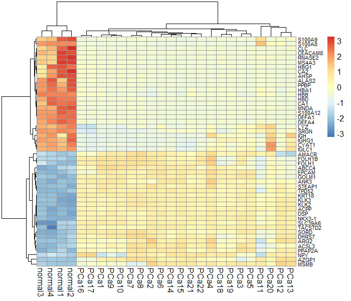
热图

install.packages("pheatmap")
library(pheatmap)
diff1<-read.csv(file="result.diff.csv",header=TRUE,sep=",")
#取上调基因、下调基因各25个
#diff2<-diff1[order(diff1$logFC)[1:25],]
#diff3<-diff1[order(diff1$logFC,decreasing= T)[1:25],]
#diff4<-rbind(diff2,diff3)
gene_expr<-read.csv(file="data.exprs3.clear.csv",header=TRUE,sep=",")
gene_expr1<-gene_expr[gene_expr$gene_symbol  %in% diff1$X,]
rownames(gene_expr1)<-gene_expr1$gene_symbol
gene_expr1<-gene_expr1[,-c(1,28)]
#名字太长
#rownames(gene_expr1)<-unlist(lapply(strsplit(rownames(gene_expr1),split = " /// "), function(x) x[1]))
gene_expr1<-as.matrix(gene_expr1)
pheatmap(gene_expr1, scale = "row", clustering_distance_row = "correlation", fontsize=12, fontsize_row=12)